Unified optimization function

I_optimx is rich of functionality, but with a low computing performance. Some basic optimization functions are unified here, with some input and output format.

• opt_ncminf General-Purpose Unconstrained Non-Linear Optimization, see ucminf::ucminf().

• opt_nlminb Optimization using PORT routines, see stats::nlminb().

• opt_nlm Non-Linear Minimization, stats::nlm().

• opt_optim General-purpose Optimization, see stats::optim().

opt_ucminf(par0, objective, ...)

opt_nlm(par0, objective, ...)

opt_optim(par0, objective, method = "BFGS", ...)

opt_nlminb(par0, objective, ...)

Arguments

par0

Initial values for the parameters to be optimized over.

objective

A function to be minimized (or maximized), with first argument the vector of parameters over which minimization is to take place. It should return a scalar result.

...

other parameters passed to objective.

method

optimization method to be used in p_optim. See stats::optim().

Value

• convcode: An integer code. 0 indicates successful convergence. Various methods may or may not return sufficient information to allow all the codes to be specified. An incomplete list of codes includes

  • 1: indicates that the iteration limit maxit had been reached.

  • 20: indicates that the initial set of parameters is inadmissible, that is, that the function cannot be computed or returns an infinite, NULL, or NA value.

  • 21: indicates that an intermediate set of parameters is inadmissible.

  • 10: indicates degeneracy of the Nelder–Mead simplex.

  • 51: indicates a warning from the "L-BFGS-B" method; see component message for further details.

  • 52: indicates an error from the "L-BFGS-B" method; see component message for further details.

  • 9999: error

• value: The value of fn corresponding to par

• par: The best parameter found

• nitns: the number of iterations

• fevals: The number of calls to objective.

See also

optim_pheno(), I_optim()

Examples

library(phenofit)
library(ggplot2)
library(magrittr)
library(purrr)
#> 
#> Attaching package: ‘purrr’
#> The following object is masked from ‘package:magrittr’:
#> 
#>     set_names
library(data.table)
#> 
#> Attaching package: ‘data.table’
#> The following object is masked from ‘package:purrr’:
#> 
#>     transpose

# simulate vegetation time-series
fFUN = doubleLog_Beck
par  = c( mn  = 0.1 , mx  = 0.7 , sos = 50 , rsp = 0.1 , eos = 250, rau = 0.1)
par0 = c( mn  = 0.15, mx  = 0.65, sos = 100, rsp = 0.12, eos = 200, rau = 0.12)

t    <- seq(1, 365, 8)
tout <- seq(1, 365, 1)
y <- fFUN(par, t)

optFUNs <- c("opt_ucminf", "opt_nlminb", "opt_nlm", "opt_optim") %>% set_names(., .)
opts <- lapply(optFUNs, function(optFUN){
    optFUN <- get(optFUN)
    opt    <- optFUN(par0, f_goal, y = y, t = t, fun = fFUN)
    opt$ysim <- fFUN(opt$par, t)
    opt
})

# visualization
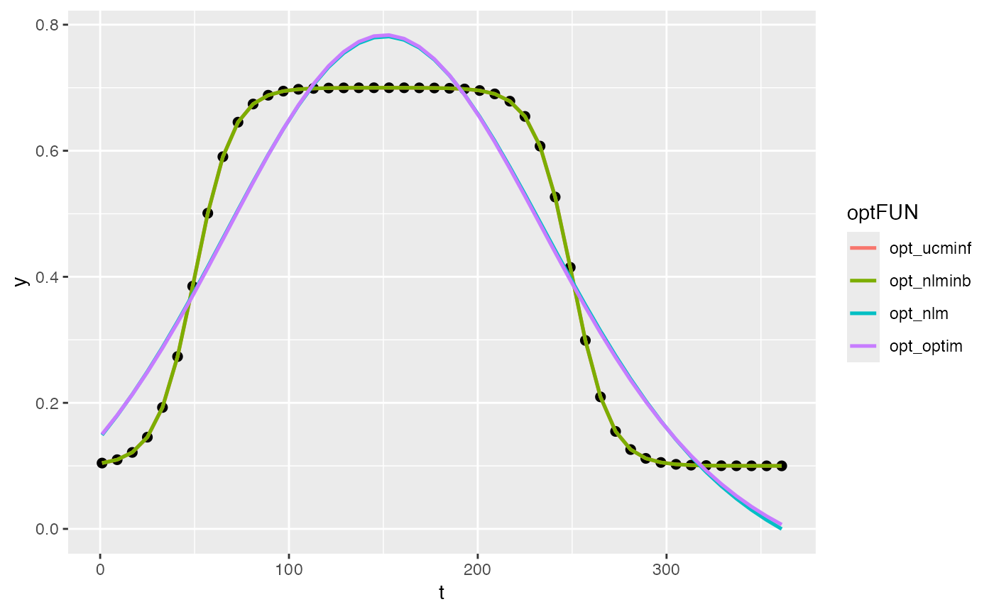
df   <- map(opts, "ysim") %>% as.data.table() %>% cbind(t, y, .)
pdat <- data.table::melt(df, c("t", "y"), variable.name = "optFUN")

ggplot(pdat) + 
    geom_point(data = data.frame(t, y), aes(t, y), size = 2) + 
    geom_line(aes(t, value, color = optFUN), linewidth = 0.9)