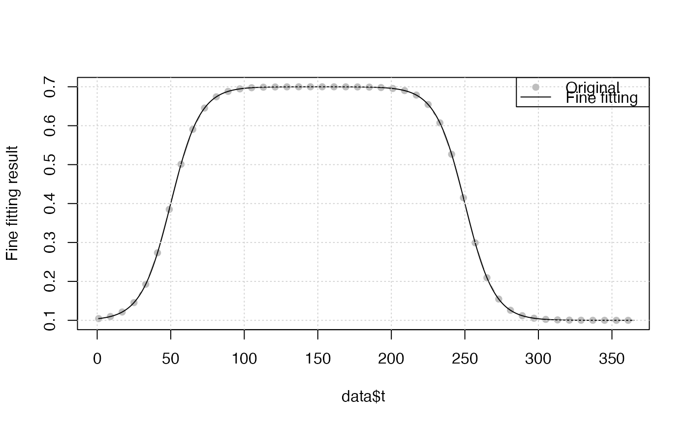
Fine curve fitting function is used to fit vegetation time-series in every growing season.
FitDL.Zhang(y, t = index(y), tout = t, method = "nlm", w, type = 1L, ...)

FitDL.AG(y, t = index(y), tout = t, method = "nlminb", w, type = 1L, ...)

FitDL.AG2(y, t = index(y), tout = t, method = "nlminb", w, type = 1L, ...)

FitDL.Beck(y, t = index(y), tout = t, method = "nlminb", w, type = 1L, ...)

FitDL.Elmore(y, t = index(y), tout = t, method = "nlminb", w, type = 1L, ...)

FitDL.Gu(y, t = index(y), tout = t, method = "nlminb", w, type = 1L, ...)

FitDL.Klos(y, t = index(y), tout = t, method = "BFGS", w, type = 1L, ...)
Arguments
- y
input vegetation index time-series.
- t
the corresponding doy(day of year) of y.
- tout
the time of output curve fitting time-series.
- method
method passed to
optimxoroptimfunction.- w
weights
- type
integer,
1or-11: trough-to-trough curve fitting-1: peak-to-peak curve fitting
- ...
other paraters passed to
optim_pheno().
Value
tout: The time of output curve fitting time-series.zs: Smoothed vegetation time-series of every iteration.ws: Weights of every iteration.par: Final optimized parameter of fine fitting.fun: The name of fine fitting.
References
Beck, P.S.A., Atzberger, C., Hogda, K.A., Johansen, B., Skidmore, A.K., 2006. Improved monitoring of vegetation dynamics at very high latitudes: A new method using MODIS NDVI. Remote Sens. Environ. https://doi.org/10.1016/j.rse.2005.10.021.
Elmore, A.J., Guinn, S.M., Minsley, B.J., Richardson, A.D., 2012. Landscape controls on the timing of spring, autumn, and growing season length in mid-Atlantic forests. Glob. Chang. Biol. 18, 656-674. https://doi.org/10.1111/j.1365-2486.2011.02521.x.
Gu, L., Post, W.M., Baldocchi, D.D., Black, TRUE.A., Suyker, A.E., Verma, S.B., Vesala, TRUE., Wofsy, S.C., 2009. Characterizing the Seasonal Dynamics of Plant Community Photosynthesis Across a Range of Vegetation Types, in: Noormets, A. (Ed.), Phenology of Ecosystem Processes: Applications in Global Change Research. Springer New York, New York, NY, pp. 35-58. https://doi.org/10.1007/978-1-4419-0026-5_2.
https://github.com/cran/phenopix/blob/master/R/FitDoubleLogGu.R
Examples
# simulate vegetation time-series
t    <- seq(1, 365, 8)
par  <- c(mn = 0.1, mx = 0.7, sos = 50, rsp = 0.1, eos = 250, rau = 0.1)
y    <- doubleLog.Beck(par, t)
data <- data.frame(t, y)
# methods <- c("AG", "Beck", "Elmore", "Gu", "Zhang")
tout <- seq(1, 365, 1)
r <- FitDL.Elmore(y, t, tout)

plot(r, data)

get_GOF(r, data)
#>       R2   NSE     R         RMSE pvalue n_sim
#>    <num> <num> <num>        <num>  <num> <num>
#> 1:     1     1     1 2.503802e-10      0    46
get_param(r)
#> # A tibble: 1 × 7
#>      mn    mx   sos   rsp   eos   rau    m7
#>   <dbl> <dbl> <dbl> <dbl> <dbl> <dbl> <dbl>
#> 1 0.100 0.600  50.0 0.100  250. 0.100     0